Computation of Lie Derivatives by Algorithmic Differentiation
Lie derivatives are usually computed using computer algebra software. This can result in very large expressions. We suggest an alternative approach using algorithmic of automatic differentiation.
Nonlinear Systems
Consider a nonlinear system-space system
\[\dot{\mathbf{x}}=\mathbf{f}(\mathbf{x}),\quad y=h(\mathbf{x})\]with the state vector $\mathbf{x}$, the output $y$, a vector field $\mathbf{f}:\mathbb{R}^{n}\to\mathbb{R}^{n}$ and a scalar field $ $$h:\mathbb{R}^{n}\to\mathbb{R}$. The Lie derivative $L_{\mathbf{f}}h$ of $h$ along $\mathbf{f}$ is given by
\[L_{\mathbf{f}}h(\mathbf{x})=\frac{\partial h(\mathbf{x})}{\partial\mathbf{x}}\mathbf{f}(\mathbf{x}).\]Higher order Lie derivatives are defined recursively by
\[L_{\mathbf{f}}^{k+1}h(\mathbf{x})=\frac{\partial L_{\mathbf{f}}^{k}h(\mathbf{x})}{\partial\mathbf{x}}\mathbf{f}(\mathbf{x})\quad\mbox{with}\quad L_{\mathbf{f}}^{0}h(\mathbf{x})=h(\mathbf{x}).\]The time derivative of the output of the nonlinear system can be written as
\[\dot{y}=\frac{\partial h}{\partial\mathbf{x}}\dot{\mathbf{x}}=\frac{\partial h}{\partial\mathbf{x}}\mathbf{f}(\mathbf{x})=L_{\mathbf{f}}h(\mathbf{x}).\]Similarly, we have
\[\ddot{y}=\frac{\partial L_{\mathbf{f}}h}{\partial\mathbf{x}}\mathbf{f}(\mathbf{x})=L_{\mathbf{f}}^{2}h(\mathbf{x}),\ldots,y^{(k)}=L_{\mathbf{f}}^{k}h(\mathbf{x}).\]In other words: Lie derivatives can be interpreted as time derivatives of the system’s output. Therefore, the output signal can be expanded into the Lie series
\[y(t)=\sum_{k=0}^{\infty}L_{\mathbf{f}}^{k}h(\mathbf{x}_{0})\frac{t^{k}}{k!}.\]Algorithmic/automatic differentiation
Consider a smooth map $\mathbf{F}:\mathbb{R}^{n}\to\mathbb{R}^{m}$. A given curve
\[\mathbf{x}(t)=\mathbf{x}_{0}+\mathbf{x}_{1}t+\mathbf{x}_{2}t^{2}+\cdots+\mathbf{x}_{d}t^{d}+\mathcal{O}(t^{d+1})\]with the Taylor coefficients $\mathbf{x}_0,\ldots,\mathbf{x}_d\in\mathbb{R}^{n}$ is mapped via $\mathbf{F}$ into the curve
\[\mathbf{z}(t)=\mathbf{z}_{0}+\mathbf{z}_{1}t+\mathbf{z}_{2}t^{2}+\cdots+\mathbf{z}_{d}t^{d}+\mathcal{O}(t^{d+1}),\]where the Taylor coefficients are given by
\[\mathbf{z}_{k}=\frac{1}{k!}\,\left.\frac{\partial^{k}\mathbf{z}(t)}{\partial t^{k} }\right|_{t=0}.\]There are several algorithmic differentiation packages such as ADOL-C or FADBAD++ which support the calculation of these univariate Taylor coefficients.
Computation of Lie Derivatives
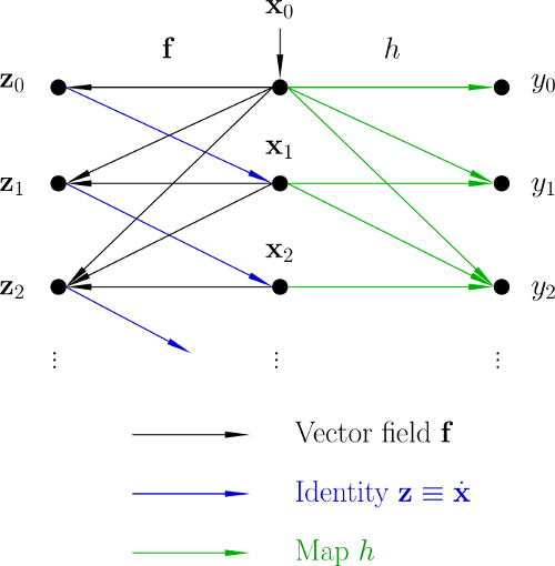
Now, we consider the following equations:
\[\begin{array}{rcl} \dot{\mathbf{x}}(t) & = & \mathbf{f}(\mathbf{x}(t))\\ \mathbf{z}(t) & = & \mathbf{f}(\mathbf{x}(t))\\ y(t) & = & h(\mathbf{x}(t)) \end{array}\]Here, $\mathbf{f}$ is treated simultaneously as a vector field of the nonlinear system and a map, which maps a curve $\mathbf{x}$ into a curve $\mathbf{z}$. These curves are related by $\mathbf{z}\equiv\dot{\mathbf{x}}$. This means
\[\mathbf{x}_{k+1}=\frac{1}{k+1}\,\mathbf{z}_{k}\quad\mbox{for}\quad k\geq0\]for the Taylor coefficients of the curves. Starting with the initial value, we can reversively compute the Tayor coefficients \(\mathbf{x}_{1},\ldots,\mathbf{x}_{d}\in\mathbb{R}^{n}\) Applying algorithmic differentiation to the map $h$, we can compute the Taylor coefficients $y_{0},\ldots,y_{d}\in\mathbb{R}$ of the output curve
\[y(t)=y_{0}+y_{1}t+y_{2}t^{2}+\cdots y_{d}t^{d}+\mathcal{O}(t^{d+1}).\]Comparing this series expansion with the above mentioned Lie series, we obtain the function values of the Lie derivatives as
\[L_{\mathbf{f}}^{k}h(\mathbf{x}_{0})=k!\, y_{k}\quad\mbox{for}\quad k=0,\ldots,d.\]These Lie derivatives are needed for nonlinear controller design by exact feedback linearization.
Data Dependencies
Publication
- Röbenack, K.; Reinschke, K. J.: The Computation of Lie Derivatives and Lie Brackets based on Automatic Differentiation.
Zeitschrift für Angewandte Mathematik und Mechnik (ZAMM), 2004, 84, 114-123 - Röbenack, K.: Computation of Lie Derivatives of Tensor Fields Required for Nonlinear Controller and Observer Design Employing Automatic Differentiation.
Proc. in Applied Mathematics and Mechanics, 2005, 5, 181-184 - Röbenack, K.; Winkler, J.; Wang, S.: LIEDRIVERS - A Toolbox for the Efficient Computation of Lie Derivatives Based on the Object-Oriented Algorithmic Differentiation Package ADOL-C.
In: Proc. of the 4th International Workshop on Equations-Based Object-Oriented Modeling Languages and Tools (EOOLT 2011). Zurich, Switzerland, September 5, 2011. ISSN: 1650-3686.